Chapter 5 — EDSMAC4 Tutorial

Description

This tutorial illustrates a very common use of EDSMAC4, that is, to perform a time-distance study to evaluate accident avoidability.

Using HVE to execute this event further illustrates the power of visualization: while the EDSMAC4 event tells us the time available to avoid a crash, the visualization actually shows us. The capability to visualize is inherent to any HVE simulation.

This tutorial is a continuation of the EDCRASH Tutorial, wherein the initial vehicle velocities were estimated. You may wish to review that tutorial before continuing.

Like all EDSMAC4 events, the procedure involves the following basic steps:

• Create the vehicle(s)
• Create the environment
• Execute the EDSMAC4 event
• Review the EDSMAC4 output reports

NOTE: It is assumed that either HVE-2D or HVE is up and running, and that the user is familiar with the program's basic features, such as using dialogs and viewers, as well as the Editors. The purpose of this tutorial is to illustrate those features while setting up and executing an EDSMAC4 event.

Getting Started

NOTE: If you just finished the EDCRASH Tutorial, you have already created your vehicles and environment and may proceed directly to Creating Events, below. The same suggestion applies if you already did the EDCRASH Tutorial and saved the case; if so, simply open that case and skip ahead.

As in other tutorials, before we get started, let's set the user options so we're all starting on the same page.

NOTE: In HVE-2D, all options simply affect the appearance in a viewer during Event or Playback mode. However, in HVE, AutoPosition affects the data used in the analysis. For example, if AutoPosition is On, the vehicle position conforms to the local surface; otherwise, the position is set by the Position/Velocity dialog. Obviously, the resulting difference in initial conditions could substantially change the event.

NOTE: Some of the following options are "toggles" that switch between two different modes. Make sure these options are set correctly.

To set the initial user options, choose the following from the Options Menu:

• ON: Show Key Results
• OFF: Show Axes
• OFF: Show Contacts
• OFF: Show Belt Anchors
• OFF: Show Velocity Vectors
• ON: Show Skidmarks
• OFF: Show Targets
• ON: AutoPosition
• Units equals S.I.

NOTE: As we'll see when we create the environment, our EDSMAC4 Tutorial takes place in Australia; thus, we require metric units.

• Render Options:
• Show Humans as Actual
• Show Vehicles as Actual
• Phong Render Method
• Complexity equals Object
• Render Quality equals 5
• Texture Quality equals 1
• Anti-aliasing equals 1

The remaining options will automatically initialize to their default conditions. We're now ready to proceed with the tutorial.

Creating the Vehicles

Let's add the vehicles to our case. The first vehicle is a white, 1996 Ford Escort 2-Door Hatchback; the second vehicle is a dark red 1995 Nissan Sentra 4-Door Sedan. Let's add the first vehicle:

1. If the Vehicle Editor is not the current editor, choose Vehicle Mode. The Vehicle Editor is displayed.
2. Click Add New Object. The Vehicle Information dialog is displayed. The Vehicle Information dialog allows the user to select the basic vehicle attributes according to Type, Make, Model, Year and Body Style.

NOTE: The Vehicle Information dialog also allows you to edit the Driver Location, Engine Location, Number of Axles and Drive Axle(s). These options are assigned default values for each vehicle. For our tutorial, only driver location must be edited.

1. Using the option buttons, choose the following vehicle from the database:
2. Type = Passenger Car
3. Make = Ford
4. Model = Escort
5. Year = 1991-1996
6. Body Style = 2-Door Hatchback
7. Source Database = Tutorial.db
8. Driver Location = Right
9. Click OK to add the Ford Escort to the Active Vehicles list.

The Ford Escort is added to the case. Next, let's add the Nissan Sentra.

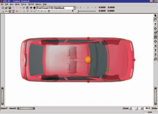
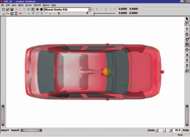Figure 5-1: Ford Escort (above) and Nissan Sentra (below).

1. Click Add New Object. The Vehicle Information dialog is displayed.
2. Using the option buttons, choose the following vehicle from the database:
3. Type = Passenger Car
4. Make = Nissan
5. Model = Sentra
6. Year = 1995-1999
7. Body Style = 4-Door
8. Source Database = Tutorial.db
9. Driver Location = Right
10. Click OK to add the Nissan Sentra to the Active Vehicles list.

We now have the vehicles required for our study, as shown in Figure 5-1.

Editing the Vehicles

Next, we'll edit the vehicles to change their color and weight. In addition, we'll change the stiffness of the Nissan Sentra, using values derived from our initial reconstruction analysis.

Start by changing the color of the Ford Escort:

1. Select the Ford Escort from the Active Vehicles drop-down list, making it the current vehicle. The Ford Escort is now displayed in the Vehicle Editor.
2. Click on the CG and choose Color. The Vehicle Color dialog is displayed, showing the vehicle's current color (the small black square, or hot spot, in the color wheel) and intensity (the arrow in the intensity slider). Click on the hot spot and drag it to the center of the circle. To lighten the vehicle, click on the intensity slider and drag it to the far right end.

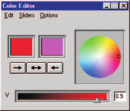Figure 5-2: Vehicle Color dialog, used for assigning the vehicle color.

NOTE: The color chip on the left shows the current color.

1. When the color is to your liking, close the dialog by clicking the close button on the upper right corner of the dialog.

NOTE: The vehicle's apparent color may be slightly misleading because the vehicle is translucent when displayed in the Vehicle Editor. The actual color will be used whenever the vehicle is displayed during Event and Playback mode.

Next, let's change the Escort's weight. Perform the following steps:

1. Click on the CG and choose Inertias. The Inertias dialog is displayed, and we're ready to change the vehicle's weight.

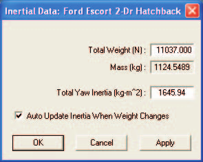Figure 5-3: Vehicle Inertias dialog, used for editing the current weight and yaw inertia (roll and pitch inertias are not used by EDSMAC4).

NOTE: The vehicle's roll, pitch and yaw moments of inertia and xz product of inertia are also displayed in the Inertias dialog; however, only the yaw inertia is used by the 3-DOF EDSMAC4 calculations.

1. In the Total Weight text field, replace the existing weight, 10283 Newtons, with the measured value, 11037 Newtons.

NOTE: The weight is entered as a force (Newtons). Mass units (kg) are calculated and displayed.

NOTE: The dialog might initially display 10283.5, or a similar number, because the weight is actually divided by the current gravity constant and stored as mass. Extra precision results when the mass is multiplied by the current gravity constant and redisplayed.

1. If not already selected, click the checkbox for Auto Update Inertia When Weight Changes.
2. Press OK to accept the weight value and update the Total Yaw Inertia of the vehicle.

The Ford Escort is now ready for use in our tutorial. Using the viewer thumb wheels and/or manipulators, pan, zoom and look at the vehicle. Note that, in HVE, the thumb wheels rotate the vehicle about the viewer axes, not the vehicle axes.

NOTE: It is important to be able to manipulate (pan, rotate and zoom) the objects in the current viewer. Refer to the User's Manual (see Window Manager Basics) for more information.

Now, let's change the color, weight and stiffness of the Nissan Sentra:

1. Click on Nissan Sentra 4-Dr in the Active Vehicles list, making it the current vehicle. The Nissan Sentra is now displayed in the Vehicle Editor.
2. Click on the CG and choose Color. The Vehicle Color dialog is displayed. The vehicle's color is fine, but we need to darken it. To darken the vehicle, click on the intensity slider and drag it to the middle of the range.
3. When the color is to your liking, close the dialog.

Next, let's change the Nissan's weight:

1. Click on the CG and choose Inertias. The Inertias dialog is displayed.
2. In the Total Weight text field, replace the existing weight, 10858 Newtons, with the measured value, 11282 Newtons.

NOTE: Again, the value displayed in the dialog may contain extra precision, for reasons explained earlier.

1. If not already selected, click the checkbox for Auto Update Inertia When Weight Changes.
2. Press OK to accept the weight value and update the Total Yaw Inertia of the vehicle.

Finally, let's change the stiffness of the vehicle. From a previous reconstruction analysis, the A and B stiffnesses were re-calculated in order to balance the forces (the technique is described in references [20] and [21]). Based on this analysis, let's enter the new values:

1. Click on the right side surface icon (red sphere). The CG to Right Side dialog is displayed.
2. Click Stiffness. The Stiffness Coefficients dialog for the right side surface is displayed.

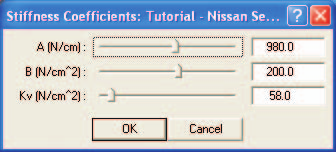Figure 5-4: Vehicle Stiffness dialog, used for editing the current A, B and KL stiffness coefficients for the current surface. Note that EDSMAC4 uses the A and B stiffness for the selected surface; earlier programs used a single value of KL for the entire vehicle.

To edit the current A and B stiffness values:

1. In the A Stiffness field, replace the current value, 175.1, with the calculated value, 980 N/cm.
2. In the B Stiffness field, replace the current value, 45.6, with the calculated value, 200 N/cm².
3. Click OK to update the stiffness.
4. Click OK again to remove the CG to Right Side dialog.

The Nissan Sentra is now ready for use in our tutorial. Using the viewer controls (thumb wheels and manipulators), view the vehicle. Now, we have both vehicles ready for our study.

Saving the Case

Now that we've created vehicles for our case, let's save the case file.

1. Click on the File menu and choose Save. The Save-as File Selection dialog is displayed.

If you began this case using the EDCRASH Tutorial, your case will be saved using the existing filename, EdcrashTutorial.

NOTE: If you started this tutorial as a new case, the Save-as dialog is displayed because the case has not been saved previously, so we need to enter a filename. Continue with the following steps.

1. In the Case Title text field, enter EDSMAC4 Tutorial, Visibility Study.

NOTE: The Case Title is displayed as a heading on all printed output reports.

1. In the Filename text field, enter Edsmac4Tutorial.
2. Click SAVE. The current case data are saved in the ../supportFiles/case subdirectory.

NOTE: Saving the file occasionally is a highly recommended practice.

Creating the Environment

Now, let's add the environment:

1. Choose Environment Mode. The Environment Editor is displayed.
2. Click on Add New Object. The Environment Information dialog is displayed.
3. Using the Location Database combo box, choose Sydney, NSW, Australia. The latitude (35.30.00S), longitude (151.10.00E) and GMT, hours from the prime meridian (+10), are displayed for the selected location.

NOTE: If Sydney were not included in your Location Database, you could add it simply by typing in a new location name, latitude, longitude and GMT.

1. Edit the name for the accident site, Blind Intersection.
2. Edit the date and time of the incident we are studying, 7/23/97 and 1330, respectively.
3. Edit the angle from true north to the earth-fixed X axis in our environment, −10 degrees.

NOTE: The Latitude, Longitude, GMT, Date/Time and angle from true north are used to position the sun in the scene. This is, of course, important because the sun is the primary light source for the scene.

1. To add the environment geometry file to our case, click on Open. The Environment Geometry File Selection dialog is displayed.
2. Click on the Files of Type option list and choose HVE Geometry Files (*.h3d). A list of environment geometry files using the .h3d file format is displayed in a list box.
3. Double-click on EdcrashEdsmacTutorial_2D.h3d to choose the environment file and remove the dialog.

NOTE: HVE users should choose the environment file EdcrashEdsmacTutorial.h3d.

1. Press OK.

The selected environment is added to our case and displayed in the Environment Viewer. Use the viewer thumb wheels to view the scene.

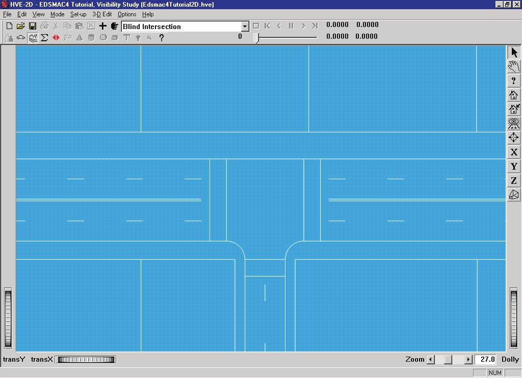
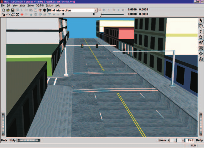Figure 5-5: Environment used for the EDSMAC4 tutorial: HVE-2D (above) and HVE (below).

Creating Events

As mentioned at the outset, this EDSMAC4 tutorial is an avoidability study in which visibility plays a key role. With this in mind, we will start simulating the event well before impact to illustrate the visibility between vehicles, as obstructed by the building on the southwest corner of the intersection.

To create the event, perform the following steps:

1. Choose Event Mode. The Event Editor is displayed.
2. Click on Add New Object. The Event Information dialog is displayed.
3. Select Ford Escort and Nissan Sentra from the Active Vehicles list. The vehicles are added to the Event Humans and Vehicles list.
4. Select EDSMAC4 from the Calculation Method options list.
5. Enter a name for the event, Visibility Study.

NOTE: The name of the calculation method will be appended to the event name, thus the complete event name will become "EDSMAC4, Visibility Study."

1. Press OK to display the event editor.

Now, we're ready to set up the event. This step involves placing the vehicles in the environment and assigning driver controls:

1. Select Ford Escort from the Event Humans & Vehicles list.
2. Choose Set-up from the menu bar, select Position/Velocity. The Escort is displayed in its initial position at the earth-fixed origin.
3. Click on the vehicle's X-Y manipulator, wait for it to turn bright yellow (indicating it has been selected), and drag it to its initial position, X = 35 m, Y = 15 m. Click the Yaw field in the Position/Velocity dialog to replace the existing value with the heading angle, 180 degrees.

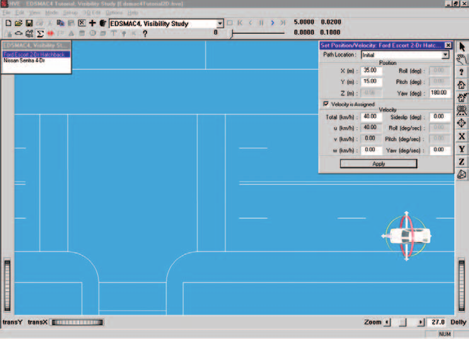Figure 5-6: Positioning the Ford Escort using the Event Editor. The manipulators can be used to drag and drop the vehicle into position. Click on the cross-bars to drag the vehicle on the road surface; click on the circular yellow ribbon to rotate the vehicle about its yaw axis.

NOTE: To select the X-Y manipulator, the viewer must be in Pick mode, as indicated by the highlighted arrow in the upper right corner of the viewer.

NOTE: Adjust the viewer by dollying back (using the Dolly thumb wheel) until you can see the entire intersection.

NOTE: Be sure to keep the mouse button depressed while you drag the manipulators.

NOTE: If you can't position the vehicle at the exact coordinates, simply enter them in the dialog (in fact, it's often easier to directly enter the coordinates using the dialog).

NOTE: When entering coordinates using the Position/Velocity dialog, remember to press Enter; otherwise, the values will not be assigned.

1. Click the Velocity Is Assigned checkbox. Enter the initial total velocity, 40 km/h, followed by Apply (or simply press Enter).

Next, let's enter the driver controls:

1. Choose Set-up from the menu bar, select Driver Controls. The Driver Controls dialog is displayed. The default driver control table, Steering, is also displayed for editing.

NOTE: Two Steer Table options are available: 'At Steering Wheel' and 'At Axle'. We'll use the default method, 'At Steering Wheel'.

1. Enter the values shown in Table 5-1 into the steer table:

Table 5-1: Steer table entries for the Ford Escort

Time (sec)	Steer Angle at Steering Wheel (degrees)
1.50	0.0
2.00	90.0

Next, let's assign the Brake Table for the Ford Escort:

1. Click the Brake tab on the Driver Controls dialog. The Brake dialog is displayed for the Ford Escort.

NOTE: Two Brake Table options are available: 'Available Friction' and 'Wheel Force'. We'll use the default method, 'Available Friction'.

1. Enter the Escort's brake table using the Available Friction (default) method, per Table 5-2:

Table 5-2: Brake table for Ford Escort — Friction (%/100)

Time (sec)	R/F	L/F	R/R	L/R
2.25	0.00	0.00	0.00	0.00
2.35	1.00	1.00	1.00	1.00
2.70	1.00	1.00	1.00	1.00
2.80	1.00	1.00	0.01	0.01

1. Click OK to accept the Ford Escort's steering and brake tables.

Event set-up for the Ford Escort is now complete. Let's set up the Nissan Sentra:

1. Select the Nissan Sentra from the Event Humans and Vehicles list.
2. Choose Set-up from the menu bar, select Position/Velocity. The Nissan is displayed at its initial position at the earth-fixed origin.
3. Click on the vehicle's X-Y manipulator, wait for it to turn bright yellow, and drag it to its initial position, X = 3.5 m, Y = 39 m. In the Yaw field in the Position/Velocity dialog, replace the existing value with the heading angle, −90 degrees.

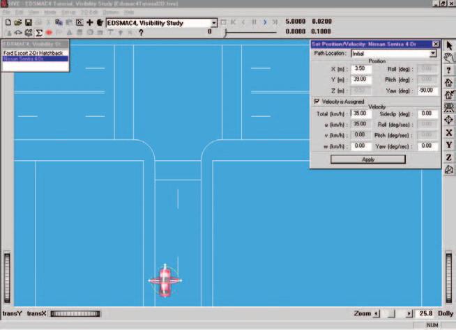Figure 5-7: Positioning the Nissan Sentra using the Event Editor. The manipulators can be used to drag and drop the vehicle into position.

1. Click the Velocity Is Assigned check box and enter the initial velocity, 35 km/h, followed by Enter.

NOTE: Remember to press Apply or Enter. Otherwise, the value will not be assigned.

The Nissan's initial position and velocity are now established. Let's enter the driver controls. In this case, there are no driver inputs, per se. However, after impact the vehicle coasts to rest, so we need to enter rolling resistances:

1. Choose Set-up from the menu bar, and select Driver Controls. The Driver Controls dialog is displayed.
2. Click the Brake tab. The Brake Table is displayed.
3. Click on the Table Is option list and choose the Available Friction option.
4. Enter the rolling resistances after impact, as shown in Table 5-3:

Table 5-3: Post-impact rolling resistances for the Nissan Sentra — Friction (%/100)

Time (sec)	R/F	L/F	R/R	L/R
2.70	0.00	0.00	0.00	0.00
2.80	0.20	0.20	0.01	0.01

1. Press OK to accept the table.

This event lasts more than 5 seconds. To prevent premature termination, let's increase the default maximum simulation time:

1. Click on the Options menu and choose Simulation Controls. The Simulation Controls dialog is displayed.
2. Edit the Maximum Time, changing it from 5 to 10 seconds.
3. Press OK to update the simulation controls.

Now, we're ready to set the camera view for the event. Let's first view the sequence from a good overall vantage point:

• Use the viewer controls (thumb wheels, zoom slider and direct hand-in-viewer manipulator) to set the view similar to that shown in Figure 5-8. (In HVE-2D, set the view to an overhead view that contains both vehicles at their initial positions.)

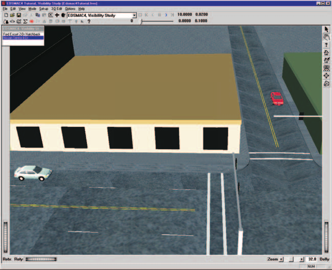Figure 5-8: Overall view of the scene after event set-up is complete.

Next, let's set up the Key Results windows:

1. If Key Results windows are not displayed, choose Show Key Results from the Options menu.
2. Drag the Key Results windows to a convenient location, where they do not block the view but still allow us access to the viewer thumb wheel controls (in case we want to change the view).

Now, we're ready to execute the event:

• Using the Event Controller, press Play to execute the event.

Watch as the vehicles approach each other, collide, and roll to their rest positions.

NOTE: You can adjust the view while the event is executing, or you can press Pause/Stop to temporarily stop the event while setting the view, then press Play to continue it.

NOTE: Remember to pay attention to the Key Results windows; in this case, you might be interested in the position and velocity of each vehicle at initial visibility.

While it is not possible to set the camera to a driver's perspective in HVE-2D (by definition a 3-dimensional operation), you can use the overhead view to determine line of sight at each timestep.

Because the issue is avoidability, let's view the sequence from several locations, including from within the vehicles, to determine what the event was actually like for each driver. Now, let's replay the sequence as viewed by the driver of the Ford Escort.

• Using the Event Controller, press Rewind.

Setting the View

HVE has additional features that we will use in this visibility study to get a driver's view of the event. Therefore, while this section of the manual is of interest to both HVE and HVE-2D users, it is written primarily for users of HVE.

A very useful feature of HVE is the ability to simulate the driver's view by attaching the camera to the vehicle in the position of the driver's head and facing in the direction of the driver's sight. In HVE-2D, the camera may also be attached to any vehicle, but the view remains straight down, essentially providing a "helicopter" view.

Let's attach the camera to the Ford:

1. Choose Set Camera from the View menu. The Camera dialog is displayed.

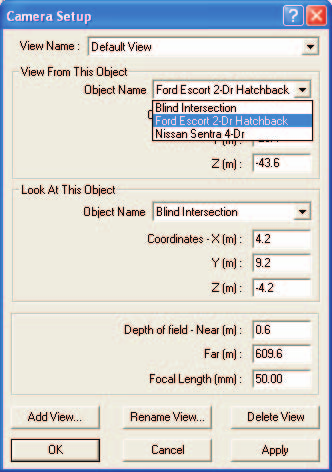Figure 5-9: HVE Set Camera dialog, used for attaching the camera to the vehicle.

1. Click on the View From This Object option list. The list displays each object in the event (Blind Intersection, Ford Escort and Nissan Sentra).
2. Choose Ford Escort from the View From This Object option list.
3. Enter the Camera coordinates, x = 0.0 m, y = 0.5 m, z = −0.6 m.

NOTE: These coordinates are vehicle-fixed, relative to the Ford Escort's coordinate system.

NOTE: These coordinates define the driver's seat location just above the roof. We placed the camera outside the car because the windshield is tinted and difficult to see through.

1. Click on the Look At This Object option list. The list displays each object in the event.
2. Choose Ford Escort from the Look At This Object option list.
3. Enter the coordinates, x = 10.0 m, y = −2.5 m, z = −0.6 m.

NOTE: These coordinates are also relative to the Ford Escort, and define a view angle looking forward and to the left, as shown in Figure 5-10.

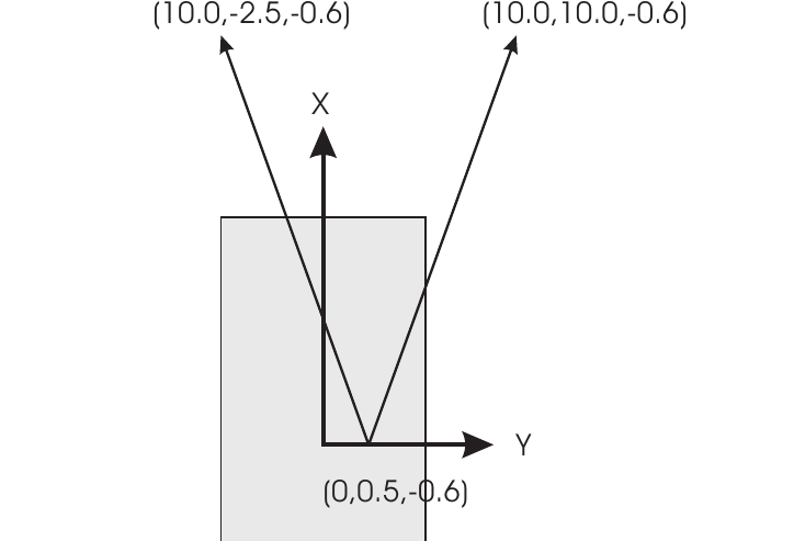Figure 5-10: Relationship between the camera position and picture center coordinates.

In HVE-2D, the view is restricted to the straight-down "helicopter" view, so there is no Look At This Object list available on the HVE-2D Camera Setup dialog.

1. Press OK to assign the new camera position.

The viewer now shows the scene as viewed from the Ford Escort. Now we're ready to see how the accident occurred from the Ford driver's perspective.

• Press Play to view the accident sequence from the Ford driver's perspective.

Watch as the Nissan becomes visible at t = 1.2 seconds. Noting from the steer table that the Ford's driver began steering at t = 1.5 seconds and began braking at t = 2.25 seconds, we can draw some conclusions regarding the driver's perception/reaction time.

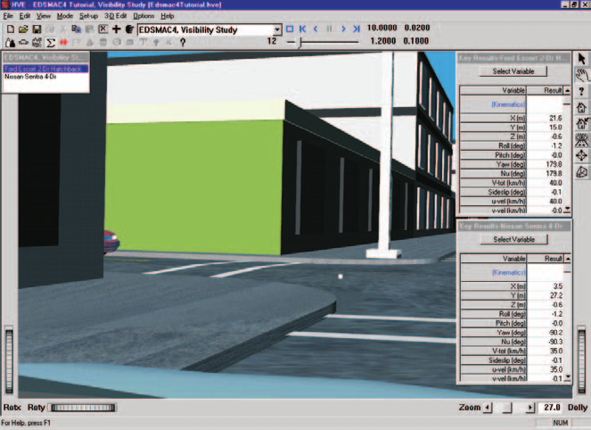Figure 5-11: Accident sequence as viewed from the driver's position in the Ford Escort at t = 1.2 seconds; the Nissan is just becoming visible.

Allow the event to run to completion.

Next, we can repeat the above steps for the driver of the Nissan Sentra:

1. Choose Set Camera from the View menu. The Camera dialog is displayed.
2. Click on the View From This Object option list and choose Nissan Sentra.
3. The Camera coordinates for the Ford Escort are acceptable for the Nissan as well.
4. Click on the Look At This Object option list and choose Nissan Sentra.
5. Enter the coordinates, x = 10.0 m, y = 10.0 m, z = −0.6 m.

NOTE: These coordinates are also vehicle-fixed, this time relative to the Nissan Sentra, and define a view angle looking forward and to the right.

1. Press OK to assign the new camera position.

Now we're ready to see how the accident occurred from the Nissan driver's perspective.

• Press Play to view the accident sequence from the Nissan driver's perspective.

Watch as the Ford becomes visible at t = 1.3 seconds. Because there was no pre-impact skidding of the Nissan, we cannot draw any conclusions regarding the Nissan driver's perception/reaction time (other than there was a lack of driver response).

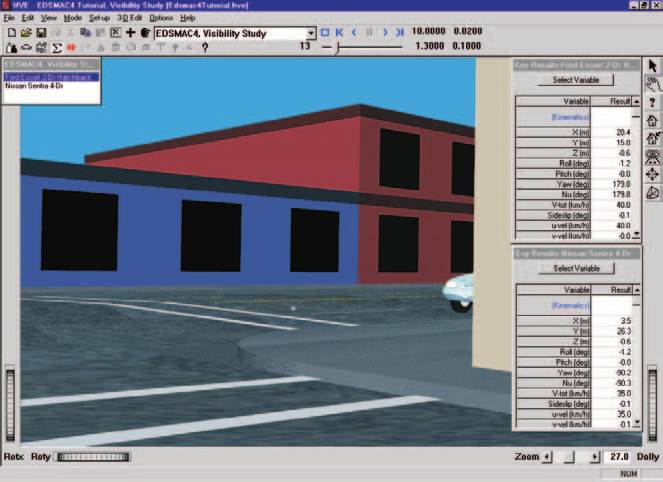Figure 5-12: Accident sequence as viewed from the driver's position in the Nissan Sentra at t = 1.3 seconds; the Ford is just becoming visible.

• Allow the event to run to completion.

You may wish to view the sequence from other perspectives or to assign the View From This Object option list to one vehicle and assign the Look At This Object option list to the other vehicle. Doing so allows the view to follow the other vehicle throughout the simulation. Use the viewer controls or the Set Camera dialog to adjust the view as necessary.

We have now completed the event.

Viewing Results

Now that we have produced our EDSMAC4 simulations, let's take a detailed look at the results. The Playback Editor is used for reviewing and printing reports for each event in the current case, as well as for producing video output.

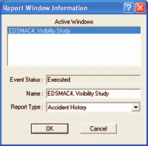Figure 5-13: Report Window Information dialog, showing the name of the event(s) in the current case.

EDSMAC4 produces the following reports:

• Accident History — A table of initial, impact, separation and final positions and velocities for each vehicle
• Damage Data — A table of damage profile coordinates, CDC, PDOF, Delta-V and Peak Acceleration for each vehicle
• Damage Profiles — A 3-D visualization of the damage to each vehicle, linked to the Playback Controller
• Driver Data — Tables of driver input to each vehicle
• Environment Data — A list of physical environment variables used by the simulation
• Event Data — A list of event-related activities such as tire blowouts or wheel displacements during the current run
• Messages — A list of messages produced by the current run
• Program Data — A table containing program control information
• Trajectory Simulation — A 3-D visualization of the event, displayed at a user-selectable time interval
• Variable Output — A table containing user-selectable, time-dependent simulation results for each vehicle
• Vehicle Data — Tables containing all of the vehicle data used by the simulation

To view the output reports, we need to be in Playback mode:

• Choose Playback Mode. The Playback Editor is displayed.

Report Windows

The reports listed above are displayed by selecting Report Windows. Each Report Window contains an individual report.

To view the reports produced by the EDSMAC4, Visibility Study event, perform the following steps:

1. Choose Playback Mode. The Playback Editor is displayed.
2. Click Add New Object. The Report Window Information dialog is displayed and includes a list of the active events (EDSMAC4, Visibility Study is the only event in this tutorial). The Report Window Information dialog also includes the user-editable Report Window Name text field and Selected Output option list.
3. Select EDSMAC4, Visibility Study from the Active Events list.
4. Click on the Select Output option list and choose any of the available reports.
5. Press OK to display the report.

The selected report will be displayed in a resizable window. The following sections illustrate the reports produced for the EDSMAC4, Visibility Study event.

NOTE: If you are using HVE, the difference in the environment geometry will cause very slight differences in the results.

Accident History

The Accident History report displays the positions and velocities for each vehicle at key times (Start of Run, Impact, Separation and Final/Rest) during the run.

To view the Accident History report: click Add New Object, select EDSMAC4, Visibility Study from the Active Events list, choose Accident History from the Select Output option list, and press OK.

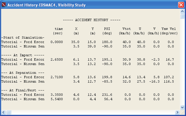Figure 5-14: Accident History Report for EDSMAC4, Visibility Study.

Damage Data

The Damage Data report displays a table of collision vector results for each vehicle. The collision vectors determine the total force on each vehicle. In addition, the endpoints of the collision vectors define the damage profile. The collision vectors are displayed both in cylindrical coordinates (RHO, PSI) and Cartesian coordinates (x,y).

Following the table of collision vectors, the Damage Ranges are displayed. The Damage Ranges report includes the beginning and ending point for each damaged region on the exterior (up to 10 regions may be displayed for each vehicle), followed by the CDC, PDOF, Delta-V and Peak Acceleration for each damage region.

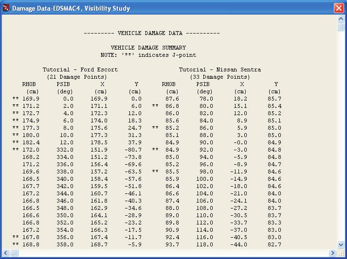
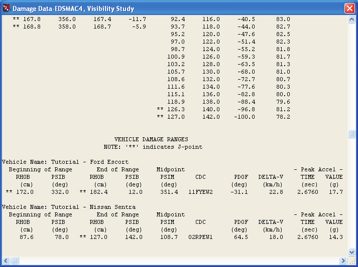Figure 5-15: Damage Data Report for EDSMAC4, Visibility Study.

To view the Damage Data report: click Add New Object, select EDSMAC4, Visibility Study, choose Damage Data from the Select Output option list, and press OK.

Damage Profiles

The Damage Profiles report provides a 3-D visual representation of the damage to each vehicle. This report is linked to the Playback Controller through the Trajectory Simulation. Therefore, in order to see any damage in the Damage Profiles report window, you must first open a Trajectory Simulation for the event.

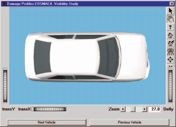Figure 5-16: Damage Profile Report for Nissan Sentra in EDSMAC4, Visibility Study.

To view the Damage Profiles report: click Add New Object, select EDSMAC4, Visibility Study, choose Damage Profiles from the Select Output option list, and press OK. With a Trajectory Simulation also open, use the Playback Controller to view the damage to each vehicle dynamically.

Driver Data

All driver input that was entered in the Event Editor is reported in the Driver Data output report.

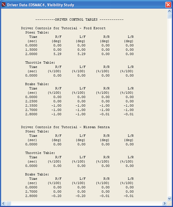Figure 5-17: Driver Data Report for EDSMAC4, Visibility Study.

To view the Driver Data report: click Add New Object, select EDSMAC4, Visibility Study, choose Driver Data from the Select Output option list, and press OK.

Environment Data

The Environment Data output report gives the values of the physical environment variables used by the simulation.

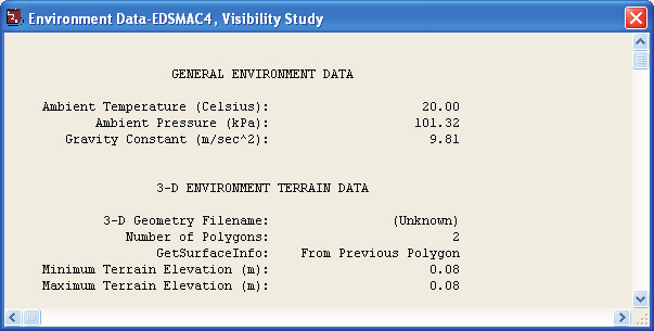Figure 5-18: Environment Report for EDSMAC4, Visibility Study.

To view the Environment Data report: click Add New Object, select EDSMAC4, Visibility Study, choose Environment Data from the Select Output option list, and press OK.

Event Data

Event-related activities such as wheel displacements or tire blowouts are reported in the Event Data report.

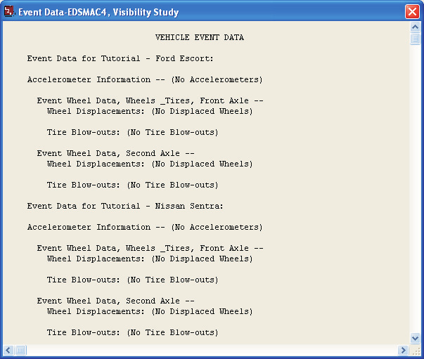Figure 5-19: Event Data Report for EDSMAC4, Visibility Study.

To view the Event Data report: click Add New Object, select EDSMAC4, Visibility Study, choose Event Data from the Select Output option list, and press OK.

Messages

EDSMAC4 produces several messages, depending on the outcome of the run. For a complete list and explanation of these messages, refer to Chapter 6.

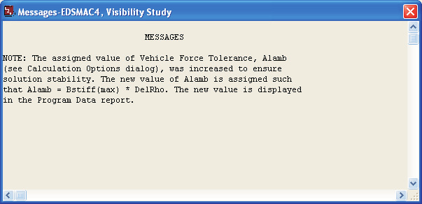Figure 5-20: Messages Report for EDSMAC4, Visibility Study.

To view the Messages report: click Add New Object, select EDSMAC4, Visibility Study, choose Messages from the Select Output option list, and press OK.

Program Data

The Program Data report displays the simulation controls (integration time steps and termination conditions), collision parameters used by the EDSMAC4 collision algorithm and the hard-coded values (RHOB Tests) used to determine if a vector passes through the end (front or back) or side (left or right).

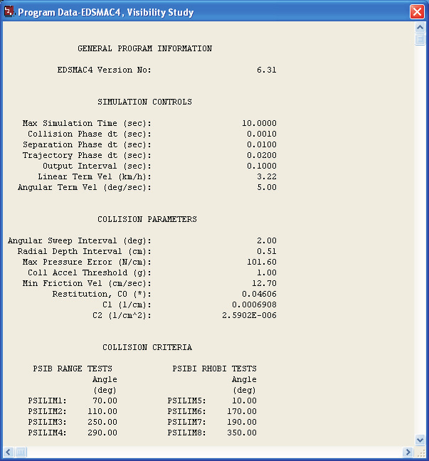Figure 5-21: Program Data Report for EDSMAC4, Visibility Study.

To view the Program Data report: click Add New Object, select EDSMAC4, Visibility Study, choose Program Data from the Select Output option list, and press OK.

Trajectory Simulation

The Trajectory Simulation report is a dynamic visualization, much like the Event mode viewer, controlled by the Playback Controller.

NOTE: A significant difference between the simulation in the Event Editor and the Playback Editor is that no calculations take place in Playback mode.

To view the Trajectory Simulation: click Add New Object, select EDSMAC4, Visibility Study, choose Traj Sim from the Select Output option list, and press OK. The Trajectory Simulation viewer is displayed with the vehicles shown at their initial positions.

During Event mode, HVE users changed the camera's View From This Object position to the Nissan. The Playback Editor inherits the camera position from Event mode, so it's still attached to the Nissan. Before we view the trajectory simulation, we will change the view back to the environment:

1. Choose Set Camera from the View menu. The Camera dialog is displayed.
2. Click on the View From This Object option list and choose Blind Intersection. Enter the desired camera coordinates, X = 50.0 m, Y = 10.0 m, Z = −3.5 m.
3. Click on the Look At This Object option list and choose Blind Intersection. Enter the desired picture center coordinates, X = 0.0 m, Y = 8.0 m, Z = 0.0 m.
4. Press OK to update the camera position.

The view is now looking down the street. To visualize the motion, perform the following steps:

1. Click Play (single right-arrow). The simulation begins and is displayed at the current Playback output interval.
2. Click Pause. The simulation stops.
3. Click Reverse (single left-arrow). The simulation plays in reverse.
4. Click Pause. The simulation stops.
5. Click Rewind (left arrow with bar). The simulation returns to the start.
6. Click Advance to End (right arrow with bar). The simulation advances to the end of the run.

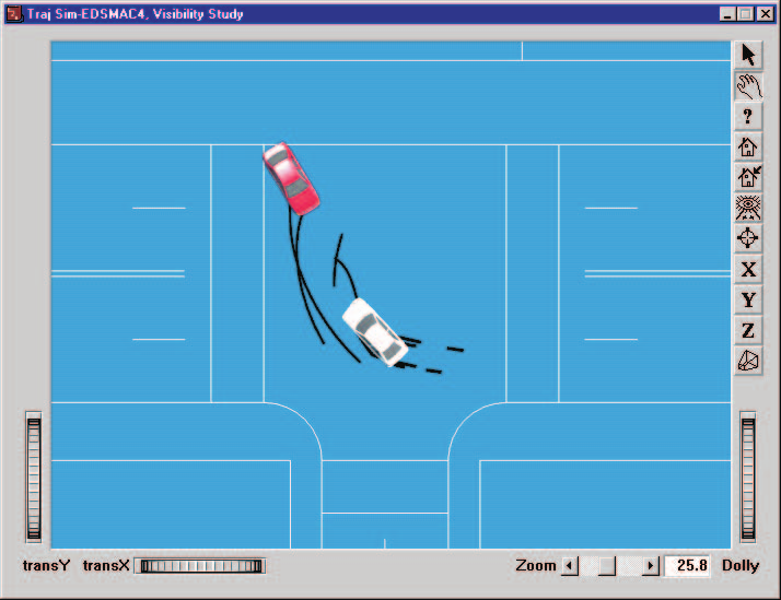
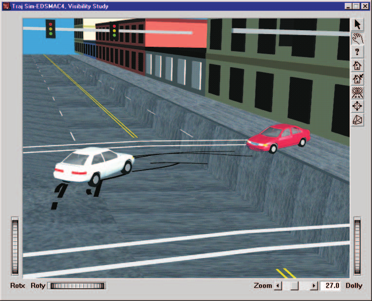Figure 5-22: Trajectory Simulation for EDSMAC4, Visibility Study, displaying the crash sequence at the end of the event (HVE-2D above, HVE below). In the lower figure, the Nissan has come to rest on the sidewalk after mounting the curb.

Variable Output

The Variable Output table displays all the time-dependent results computed by EDSMAC4. To view the Variable Output report: click Add New Object, select EDSMAC4, Visibility Study, choose Variable Output from the Select Output option list, and press OK.

The Variable Output report is displayed for the EDSMAC4, Visibility Study event. The next step is to select the time-dependent results we wish to display in the table.

Variable Selection

The purpose of our EDSMAC4 study is to evaluate the avoidability of the accident based on speeds and visibility. To document the path positions as a function of time, let's select the position, velocity and acceleration from the Variable Selection dialog.

1. Click on Select Variables in the Variable Output window. The Variable Selection dialog is displayed.

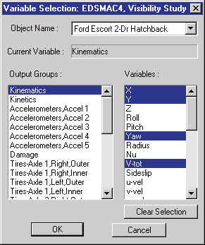Figure 5-23: Variable Selection dialog.

The Object Name option list displays the first vehicle, Ford Escort. The Kinematics output group is the default selection and the Kinematics Variables list is displayed. Let's add X, Y, Yaw, Vtotal and Accel total:

1. Select X, Y, Yaw, V-tot and Acc-tot from the list.

Next, let's add the same parameters for the Nissan Sentra:

1. Click on the Object Name option list and choose Nissan Sentra 4-Dr. The Kinematics variable list is displayed.
2. Select X, Y, Yaw, V-tot and Acc-tot from the list.

NOTE: Feel free to add additional variables to the Variable Output window.

1. Press OK to add the selected variables to the Variable Output window.

The Variable Output report for the EDSMAC4, Visibility Study event now includes position, velocity and acceleration for both vehicles, plus any other variables you may have added.

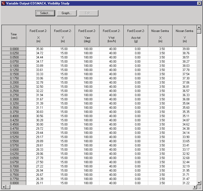Figure 5-24: Variable Output report for EDSMAC4, Visibility Study.

Vehicle Data

The Vehicle Data report displays the vehicle data, tire data and driver tables for each vehicle in the event.

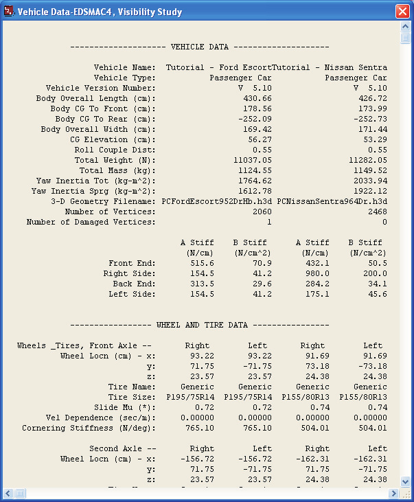Figure 5-25: Vehicle Data Report for EDSMAC4, Visibility Study.

To view the Vehicle Data report: click Add New Object, select EDSMAC4, Visibility Study, choose Vehicle Data from the Select Output option list, and press OK.

NOTE: The Vehicle Data, Damage Data and several other reports contain more information than fits into the default window size. Use the scroll bars, resize the dialog, or adjust the font size to view the entire report.

Printing

The final step is to print the above reports. Printing reports is simple. All you do is choose a report and print it. For example:

1. Click on the Variable Output — EDSMAC4, Visibility Study report window. The window is highlighted and pops to the top of the display (if it isn't there already), indicating it is the current window.
2. Click on the File menu and choose Print. The Print dialog is displayed, allowing the user to select from several available print options.

NOTE: Alternatively, you can click on the print icon in the main menu bar.

1. Press OK. The Variable Output report is printed on the system printer.

That's all there is to it! You can print any other report using the same three steps described above.

NOTE: The Print dialog provides several options. Refer to your Windows or printer manual for more information.

NOTE: For several reports it may be best to print in landscape rather than portrait mode.

NOTE: The font size of both the printed reports and screen display may be edited by clicking on the Options menu and choosing Preferences. Use the Font Size option list to change the size.

---

Previous: Chapter 4 — Calculation Method — Next: Chapter 6 — Messages

---

← Previous: Chapter 4 — Calculation Method | Index | Next: Chapter 6 — Messages →